Shape, histograms and hidden groups
Data can have tails, gaps or several groups. Two datasets can share the same mean and SD but need different decisions.
Inspect centre, spread, tail direction, peaks or gaps, and unusual values. A right tail extends toward large values; a left tail extends toward small values. Mean greater than median often accompanies a right tail, but it is a clue rather than a mathematical proof of shape. Similar mean and median or near-zero skewness does not establish normality.
A histogram groups numbers into intervals. Few wide bins may conceal two peaks; many narrow bins may exaggerate noise. Changing bins changes the picture, not the underlying observations or their mean. Compare reasonable choices and label units and valid n. For satisfaction 1-5, one bar per category preserves its discrete ordinal structure.
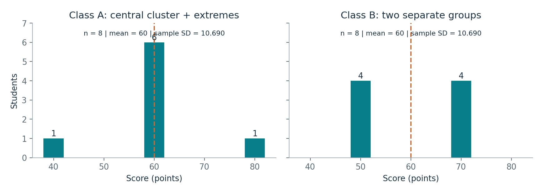
A bimodal distribution can put the overall mean between two groups where few people lie. Disaggregate using a meaningful variable and report each group's n, centre and spread. Do not infer that group membership caused the difference.
The exact Lab 2 constructions use offsets [-20,0,0,0,0,0,0,20] and [-10,-10,-10,-10,10,10,10,10]. Both have mean offset 0 and sample SD sqrt(800/7), about 10.690. The first has six central students and two extremes; the second has two groups. They can require different tutoring plans despite identical mean and SD.
Sources: W2 PDF pp. 2-60; L2 Sections 1-8. The personalised Lab 2 has 240 synthetic students, unlike the 1,200-student lecture dataset. Do not mix their numbers.
Mean, median and skewness are clues; the four plots show what they miss. Changing bins changes the picture, not the data.
The lecture's fences and whiskers become record-level checks. Programme summaries and two equal-mean/SD classes show why the whole shape matters.
The 68–95–99.7 rule is compared with observed proportions. It is an approximate model statement, not a guaranteed sample result.
Practice problems
Supplementary study questions on the lecture concepts — not verbatim exam questions. Each answer counts toward spaced review.
1. Conceptual understanding
Definitions and distinctions.
Do equal mean and median prove normality?
Changing histogram bins changes what?
2. Application
Apply the concept to a case or calculation.
A few very large durations stretch the distribution to the right. What is this?
A histogram has two separated peaks. What is a useful next check?
3. Interpretation and limitations
Evaluate assumptions and justify conclusions.
What can very wide histogram bins do?
Can two classes have identical mean and SD but different shapes?
Explain it in writing
Self-checked, not marked. Write a few sentences, then compare with the example answer. Your writing is saved as you type.
Show an example answer
Wide bins may merge two groups; narrow bins may make random bumps look important. The data are unchanged, so compare sensible choices before claiming a pattern.
Check: did you answer the question, use evidence or working, and avoid claiming more than the evidence supports?
Show an example answer
A central cluster with two extremes may need targeted individual help. Two large separated groups may need different levels of teaching for many students.
Check: did you answer the question, use evidence or working, and avoid claiming more than the evidence supports?